Last post, we built a super-simple Path-based interpolator using straight line segments. To produce smoother interpolators, without corners - typically preferred for animating motion - we’ll need correspondingly smooth generating Paths. Our primary goal in this post, then, will be:

• given a sequence of $n$ points in the cartesian plane, calculate a smooth Path passing through all points in order.

We’ll start with the simplest possible case, and generalize from there.

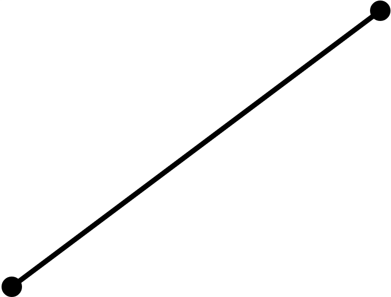
$n$ = 2

This one’s a gimme - we can use Path.lineTo(...) to connect the two given points with a straight line. While not very exciting, this curve does satisfy the smoothness condition since there are definitely no corners!

$n$ > 2

When given more than two distinct points, it’s no longer possible to connect them smoothly using straight lines only¹:

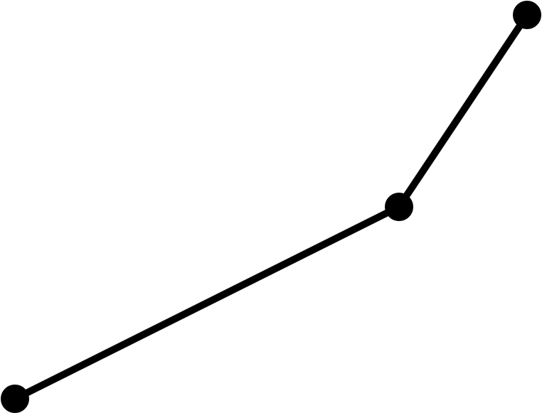
We instead need to build our Path from components with a greater number of degrees of freedom. In particular, we need to be able to specify both the end point positions and one or more derivatives of each component at those end points. That way, we can be sure that the composite curve created by joining together all our components will be smooth at the joins.

Enter Cubic Bézier Curves

Most of you will have played with Bézier curves before in consumer graphics programs. They are usually constructed in two steps:

1. fix the locations of the two end points ($P_0$ and $P_3$ in the diagram below);
2. position two control points ($P_1$ and $P_2$ in the diagram below) that completely determine the shape of the curve connecting the two end points.

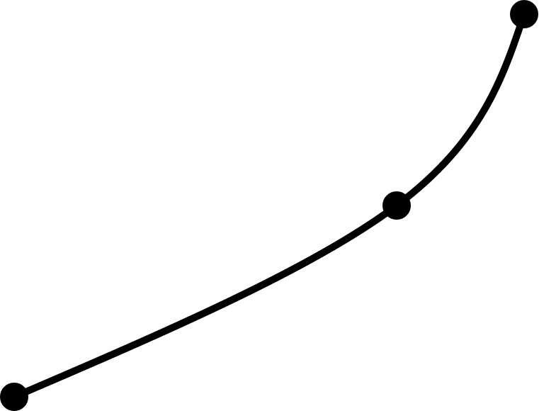
We can append a single cubic Bézier curve to an existing Path using the Path.cubicTo(...) method. But how do we make sure that we choose control points that yield a smooth composite curve? In other words, how do we ensure that our composite curve looks like this:

and not like this:

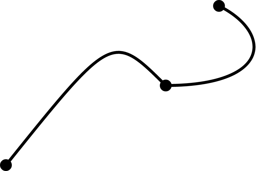
Most of the rest of this post is dedicated to figuring out how to choose the ‘right’ control points for arbitrary given end points (aka knots in Bézier curve lingo). It’s not too hairy - there’s a lot of algebra, sure, but because cubic Bézier curves can be represented as polynomials², the numbers work out nicely :). The language is fairly formal so that I can refer back to the derivations with confidence in the future. If you’re really not keen on math, you can skip ahead to the results section now.

Notation

Let $\lbrace k_i \in \mathbb{R}^m : i \in 0,\ldots,n \rbrace$ represent a collection of $n+1$ knots.

Let $\Gamma_i$ represent any cubic Bézier curve connecting $k_i$ to $k_{i+1}$ for $i \in 0,\ldots,n-1$. Each $\Gamma_i$ may then be represented by a parametric equation of the form

where $t$ ranges between $0$ and $1$, and $c_{i,0} \in \mathbb{R}^m$ and $c_{i,1} \in \mathbb{R}^m$ are the intermediate control points that determine the curvature of $\Gamma_i$.

Formal Goal

For any given collection of knots, we aim to compute control points that guarantee the composite curve $\Gamma$ formed by connecting all the individual Bézier curves $\Gamma_i$ satisfies the following conditions:

• $\Gamma$ is twice-differentiable everywhere;
• $\Gamma$ satisfies natural boundary conditions (i.e. $\Gamma’’ = 0$ at each end).

Each $\Gamma_i$ is clearly $ C^\infty $ away from the endpoints $k_i$ and $k_{i+1}$, so the first condition above is equivalent to requiring that $\Gamma$ be twice-differentiable at every knot.

The second condition is applied to fully specify the problem, leading to a unique solution and making calculations simpler.

Derivation

Note that

and

For $\Gamma$ to be $C^2$ at each interior knot, we require that

for $i \in \lbrace 1,\ldots,n-1 \rbrace$. Substituting the derivative expressions computed above, we see that these equalities are equivalent to choosing control points that satisfy

and

So far, we have $2(n-1)$ constraints for $2n$ control points. The final constraints that will uniquely determine the locations of all control points are the boundary conditions

Equivalently,

and

Eliminating $c_{i,1}$ from all these equations gives a system of $n$ equations for $\lbrace c_{i,0} : i \in 0,\ldots,n-1 \rbrace$:

Writing these equations in matrix form:

This tridiagonal system can be solved in linear time using Thomas’ Algorithm, which in this case is guaranteed to be stable since the tridiagonal matrix is diagonally dominant. Once all $c_{i,0}$ are calculated, the remaining control points $\lbrace c_{i,1} : i \in 0,\ldots,n-1 \rbrace$ are given by the following formulae:

Implementation

The following Android/Java code uses Thomas’ Algorithm to compute appropriate control points and accomplish our original goal:

given a sequence of $n$ points in the cartesian plane, calculate a smooth Path passing through all points in order.

Note that the code was written with readability, rather than performance, in mind. EPointF is a simple 2D point representation that provides some convenient componentwise operations; the definition is given below the main block of code.

package com.example;

import android.graphics.Path;

import java.util.Collection;
import java.util.List;

public class PolyBezierPathUtil {

  /**
   * Computes a Poly-Bezier curve passing through a given list of knots.
   * The curve will be twice-differentiable everywhere and satisfy natural
   * boundary conditions at both ends.
   *
   * @param knots a list of knots
   * @return      a Path representing the twice-differentiable curve
   *              passing through all the given knots
   */
  public Path computePathThroughKnots(List<EPointF> knots) {
    throwExceptionIfInputIsInvalid(knots);

    final Path polyBezierPath = new Path();
    final EPointF firstKnot = knots.get(0);
    polyBezierPath.moveTo(firstKnot.getX(), firstKnot.getY());

    /*
     * variable representing the number of Bezier curves we will join
     * together
     */
    final int n = knots.size() - 1;

    if (n == 1) {
      final EPointF lastKnot = knots.get(1);
      polyBezierPath.lineTo(lastKnot.getX(), lastKnot.getY());
    } else {
      final EPointF[] controlPoints = computeControlPoints(n, knots);

      for (int i = 0; i < n; i++) {
        final EPointF targetKnot = knots.get(i + 1);
        appendCurveToPath(polyBezierPath, controlPoints[i], controlPoints[n + i], targetKnot);
      }
    }

    return polyBezierPath;
  }

  private EPointF[] computeControlPoints(int n, List<EPointF> knots) {
    final EPointF[] result = new EPointF[2 * n];

    final EPointF[] target = constructTargetVector(n, knots);
    final Float[] lowerDiag = constructLowerDiagonalVector(n - 1);
    final Float[] mainDiag = constructMainDiagonalVector(n);
    final Float[] upperDiag = constructUpperDiagonalVector(n - 1);

    final EPointF[] newTarget = new EPointF[n];
    final Float[] newUpperDiag = new Float[n - 1];

    // forward sweep for control points c_i,0:
    newUpperDiag[0] = upperDiag[0] / mainDiag[0];
    newTarget[0] = target[0].scaleBy(1 / mainDiag[0]);

    for (int i = 1; i < n - 1; i++) {
      newUpperDiag[i] = upperDiag[i] /
          (mainDiag[i] - lowerDiag[i - 1] * newUpperDiag[i - 1]);
    }

    for (int i = 1; i < n; i++) {
      final float targetScale = 1 /
          (mainDiag[i] - lowerDiag[i - 1] * newUpperDiag[i - 1]);

      newTarget[i] =
          (target[i].minus(newTarget[i - 1].scaleBy(lowerDiag[i - 1]))).scaleBy(targetScale);
    }

    // backward sweep for control points c_i,0:
    result[n - 1] = newTarget[n - 1];

    for (int i = n - 2; i >= 0; i--) {
      result[i] = newTarget[i].minus(newUpperDiag[i], result[i + 1]);
    }

    // calculate remaining control points c_i,1 directly:
    for (int i = 0; i < n - 1; i++) {
      result[n + i] = knots.get(i + 1).scaleBy(2).minus(result[i + 1]);
    }

    result[2 * n - 1] = knots.get(n).plus(result[n - 1]).scaleBy(0.5f);

    return result;
  }

  private EPointF[] constructTargetVector(int n, List<EPointF> knots) {
    final EPointF[] result = new EPointF[n];

    result[0] = knots.get(0).plus(2, knots.get(1));

    for (int i = 1; i < n - 1; i++) {
      result[i] = (knots.get(i).scaleBy(2).plus(knots.get(i + 1))).scaleBy(2);
    }

    result[result.length - 1] = knots.get(n - 1).scaleBy(8).plus(knots.get(n));

    return result;
  }

  private Float[] constructLowerDiagonalVector(int length) {
    final Float[] result = new Float[length];

    for (int i = 0; i < result.length - 1; i++) {
      result[i] = 1f;
    }

    result[result.length - 1] = 2f;

    return result;
  }

  private Float[] constructMainDiagonalVector(int n) {
    final Float[] result = new Float[n];

    result[0] = 2f;

    for (int i = 1; i < result.length - 1; i++) {
      result[i] = 4f;
    }

    result[result.length - 1] = 7f;

    return result;
  }

  private Float[] constructUpperDiagonalVector(int length) {
    final Float[] result = new Float[length];

    for (int i = 0; i < result.length; i++) {
      result[i] = 1f;
    }

    return result;
  }

  private void appendCurveToPath(Path path, EPointF control1, EPointF control2, EPointF targetKnot) {
    path.cubicTo(
        control1.getX(),
        control1.getY(),
        control2.getX(),
        control2.getY(),
        targetKnot.getX(),
        targetKnot.getY()
    );
  }

  private void throwExceptionIfInputIsInvalid(Collection<EPointF> knots) {
    if (knots.size() < 2) {
      throw new IllegalArgumentException(
          "Collection must contain at least two knots"
      );
    }
  }

}

package com.example;

/**
 * API inspired by the Apache Commons Math Vector2D class.
 */
public class EPointF {

  private final float x;
  private final float y;

  public EPointF(final float x, final float y) {
    this.x = x;
    this.y = y;
  }

  public float getX() {
    return x;
  }

  public float getY() {
    return y;
  }

  public EPointF plus(float factor, EPointF ePointF) {
    return new EPointF(x + factor * ePointF.x, y + factor * ePointF.y);
  }

  public EPointF plus(EPointF ePointF) {
    return plus(1.0f, ePointF);
  }

  public EPointF minus(float factor, EPointF ePointF) {
    return new EPointF(x - factor * ePointF.x, y - factor * ePointF.y);
  }

  public EPointF minus(EPointF ePointF) {
    return minus(1.0f, ePointF);
  }

  public EPointF scaleBy(float factor) {
    return new EPointF(factor * x, factor * y);
  }

}

Results

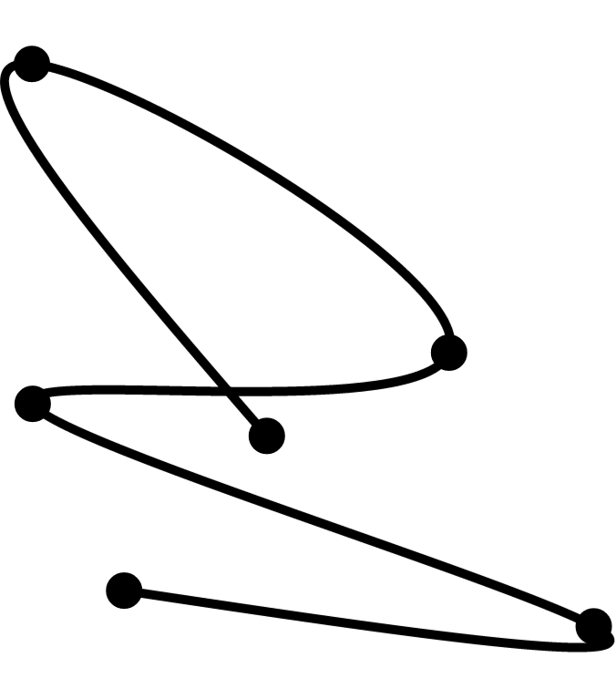
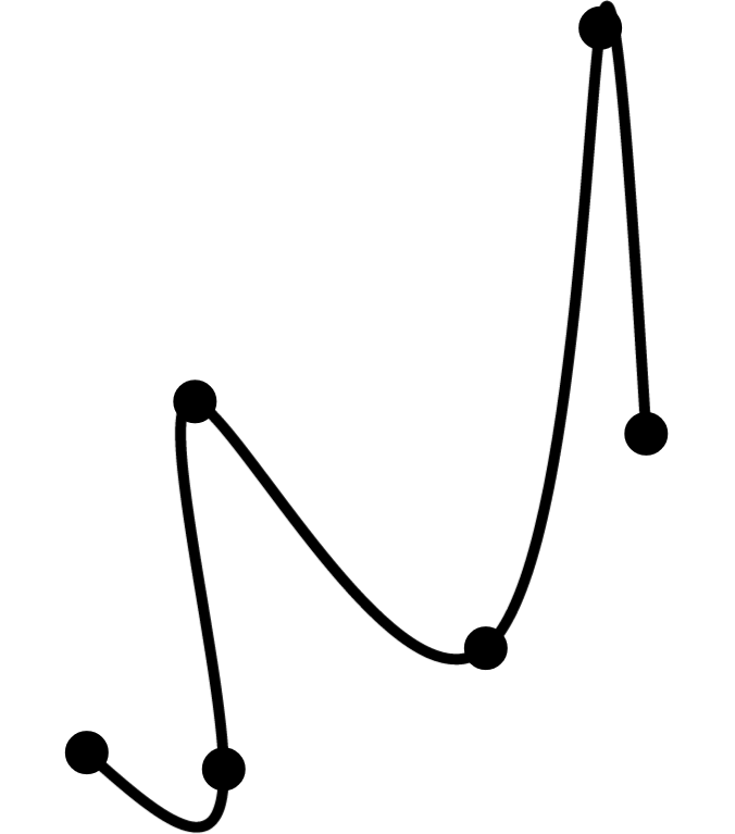
To test this implementation, I generated random points inside the square $[0,1]\times[0,1]$ and plotted the corresponding path returned by PolyBezierPathUtil. computePathThroughKnots(...). Here are a couple of examples with $n$ = 6 to convince you that everything works as expected:

Further Reading

A pleasing geometrical presentation of composite Bézier curves is provided by these lecture notes from UCLA’s Math 149: Mathematics of Computer Graphics course.

For an interesting application of Bézier curves, see the following technical articles on Square’s blog: Smooth Signatures and Smoother Signatures. Given that written letters often contain sharp corners, I would be interested to know whether Square’s algorithms could generate even better signatures if they were to switch back from cubic interpolation to linear interpolation near high-curvature regions.